Taras Kaduk: Measuring Excess Degree-Days in the Context of Location Comfort and Liveability

Taras Kaduk

Introduction

Characterization of daily air temperature as it relates to human comfort and conditions optimal for survival has many solutions. On the one hand, the mean daily, monthly, and annual air temperatures convey the necessary information with one number. However, as it is the case with many measures of central tendency, mean temperature loses a lot of important information, such as minimum and maximum values, and the range. On the other hand, minimum and maximum values inform the public of the temperature on a given day, but don’t communicate the extremity of said temperature readings well enough. Additionally, both daily min and max values, when aggregated to average minimums and average maximums, become more abstract.

Finally, a measure that is being used more frequently in recent years and is designed to communicate the dangers of climate change is the amount of days with temperature above a certain threshold. For instance, in the articles published in the United States, “days with temperature above 90°F/95°F” is frequently used (Plumer and Popovich 2017) (Climate Impact Lab 2018) (Livingston 2020). Such indicator serves its purpose relatively well, but it loses the complexity of temperature variation and extremes and potentially evens out places with different weather and temperature readings.

On the other hand, there exist indexes and calculations that reflect the weather (and temperature in particular) not in degrees or in days when a certain condition is met, but in degree-hours or degree-days, quantifying the exposure to heat energy over time. While methodologies vary based on the domain and task at hand, the key idea is to present the difference between an established baseline and actual temperature readings as area, and then to quantify that area (Thom 1952).¹

While a lot of applications of degree-hours and degree-days seem to be focused in pest control (Zalom et al. 1983), forensics (Megyesi, Nawrocki, and Haskell 2005), and vegetation research, some use of such calculations has been applied to humans (Lin et al. 2019). I propose to use this approach as an alternative approach in evaluating the exposure to excess heat and excess cold in excess heat degree-days, excess cold degree days, and total excess degree-days, where the baseline can be set as temperature optimal for human habitation, and the actual temperature curve is presented as a sine and is calculated from minimum and maximum readings for a given day. Then, quantifying excess heat, cold, and total degree-days can be accomplished with integral calculus as finding the area under the curve.

Methodology

For the purposes of this analysis, several assumptions and simplifications must be made. The daily temperature is assumed to follow a sinusoidal curve from its minimum value to its maximum value and back.² More specifically, the daily temperature curve is modeled as a cosine function, with the minimum temperature assumed at midnight and maximum temperature at noon:³

\[f(\theta) = -a \cdot cos(b\theta) + d = -\frac{({t_{max}} - {t_{min}})}{2}\cdot cos(\frac{\pi}{12}\theta) + t_{min} + \frac{(t_{max}-t_{min})}{2}\]

The baseline temperature from which the excess degree-days is calculated is assumed at 18°C, which is a mid-point between a slightly colder temperature optimal for sleep, and a slightly warmer temperature optimal for daytime activity. It needs to be pointed out that such baseline is not entirely objective, as there is no agreement on what the optimal temperature for humans is, as well as there is no consideration given to most other parameters that impact the perception of outdoor air temperature: sunlight exposure, wind, precipitation etc.

To sum up, 18°C is the baseline, and any deviation up or down from which will make a human experience of outside temperature less favorable. Along the same lines, any deviation from 18°C up or down will also make humans rely on other advances of civilization: clothing, indoor insulation, heating, air conditioning, more clothing layers, more heating etc. Thus, the higher the excess degree-days reading, the less livable the place is, or the more reliant the place is on things like air conditioning or central heating.

Excess Degree-Hours and Excess Degree-Days Calculation

The calculation of Excess Degree-Hours (or \(EDH\) for short) for the general case where the temperature curve crosses the baseline two times on a given day can be notated as:

\[EDH = \int_{0}^{\theta_1} (g(\theta) - f(\theta)) d\theta + \int_{\theta_1}^{\theta_2} (f(\theta) - g(\theta)) d\theta + \int_{\theta_2}^{24} (g(\theta) - f(\theta)) d\theta\]

where \(\theta\) is time, \(f(\theta)\) is our cosine function, \(g(\theta) = 18°C\) (the baseline), and \(\theta_1\) and \(\theta_2\) are the times at which the temperature curve crosses the baseline.

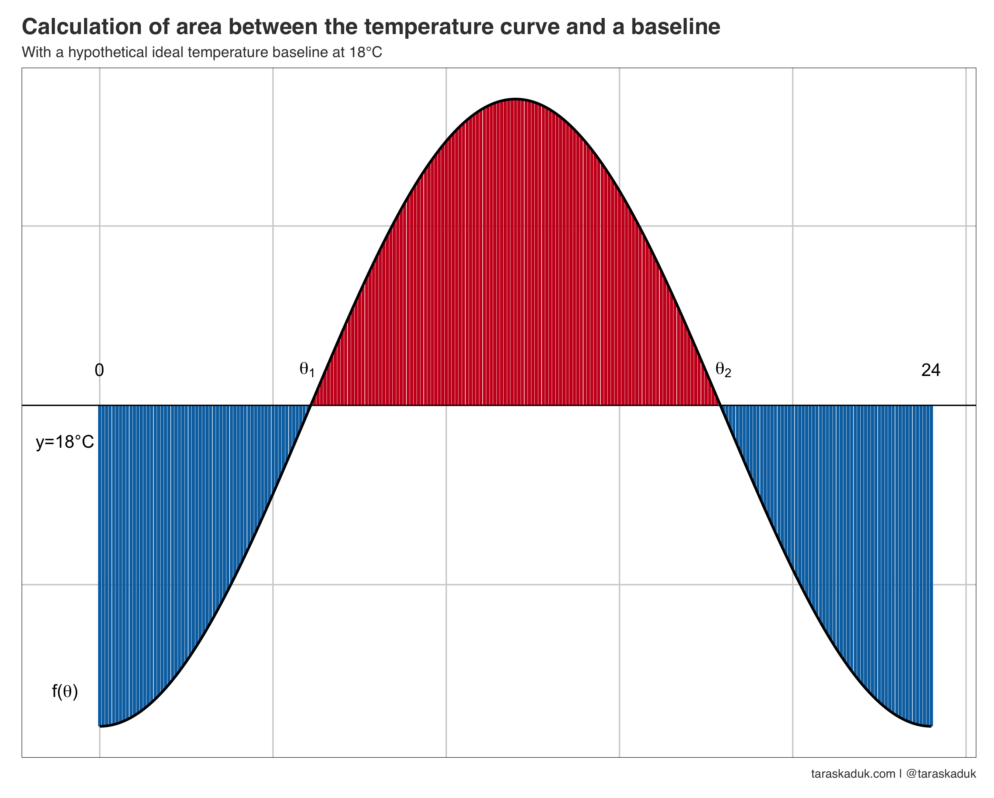
The area above the baseline stands for excess heat degree-days, and the area below the baseline - for excess cold degree-days. The sum of absolute values of both hot and cold areas will represent the total excess degree-days.

The cases when the curve stays completely above or below the baseline are special cases that require only one of the three integrals.

To get Excess Degree-Days (\(EDD\)), the \(EDH\) needs to be divided by 24: \[ EDD = \frac{EDH}{24}\]

Calculation examples

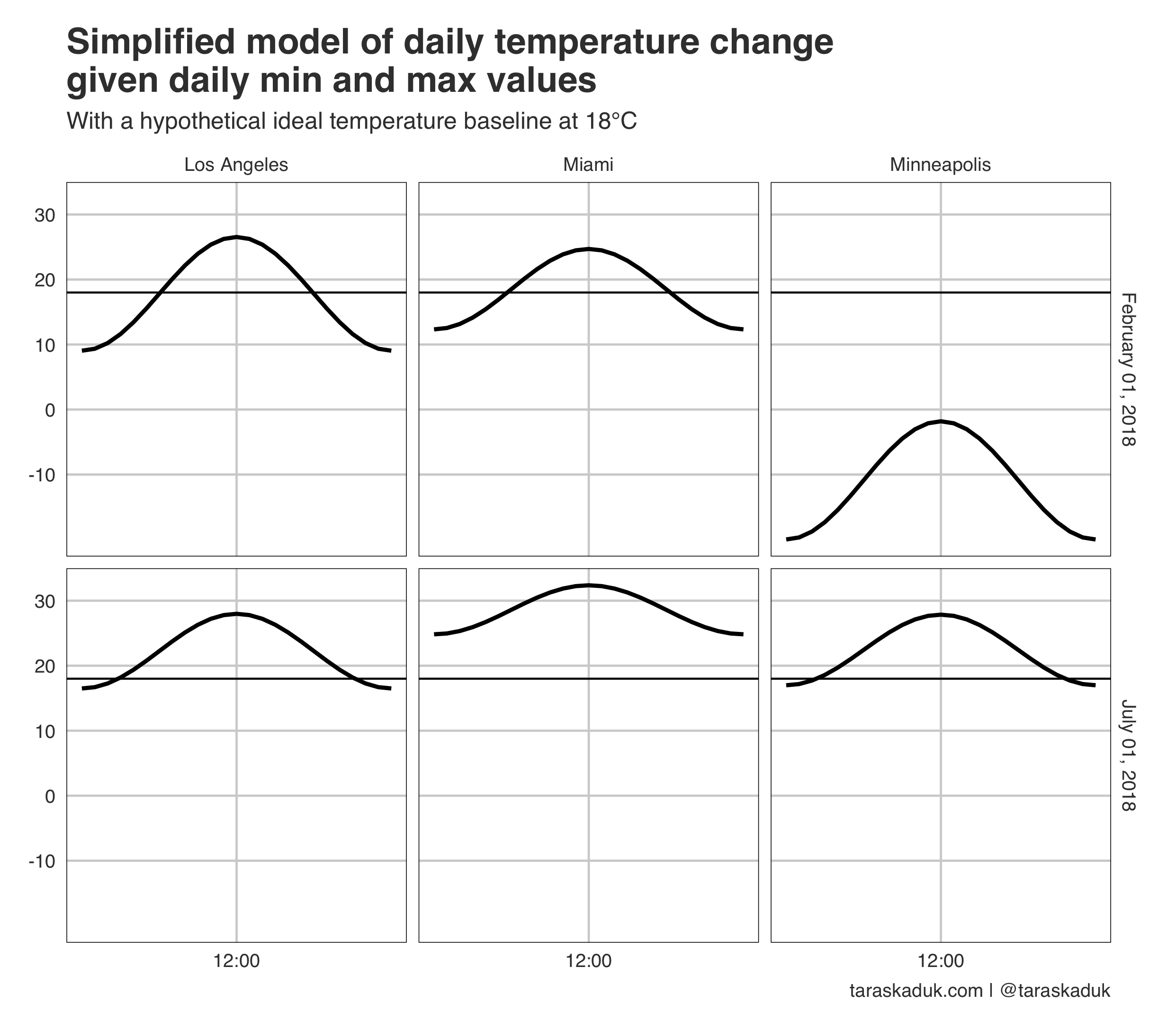
To demonstrate the way this measure works, I will use 3 cities - Los Angeles, Miami, Minneapolis - at 2 specific dates: Feb 1 and Jul 1 of 2018.

Given the min and max temperature values for each city for both days, we can model the temperature curves:

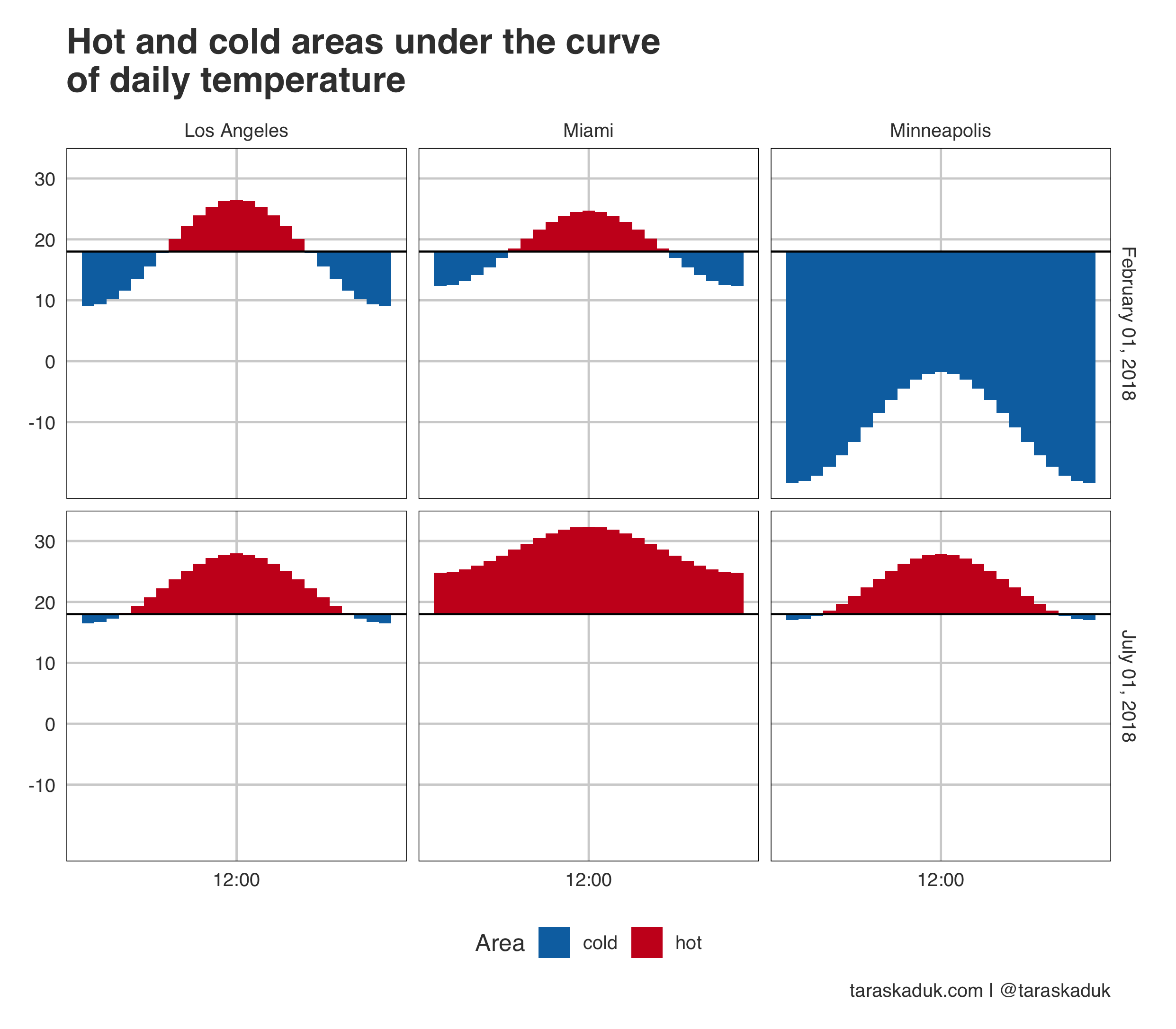
We can then proceed with calculating the area under each curve:

Looking more broadly at full year 2018, we can visualize the cumulative excess degree-hours:

Results

This article sets a theoretical basis for further practical applications. It provides another tool in the toolbox of data analysis as it relates to climate change, weather, urban comfort and livability.

My plan is to build on this work in the future, but given the time constraints, this may happen at some time in the future. Until then, I am hoping this approach will be useful to other researchers.

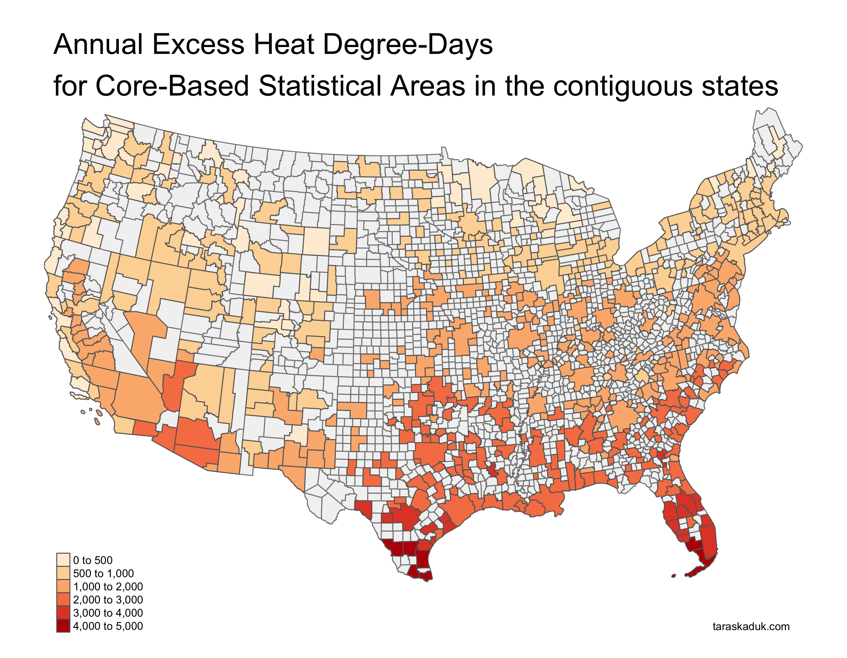
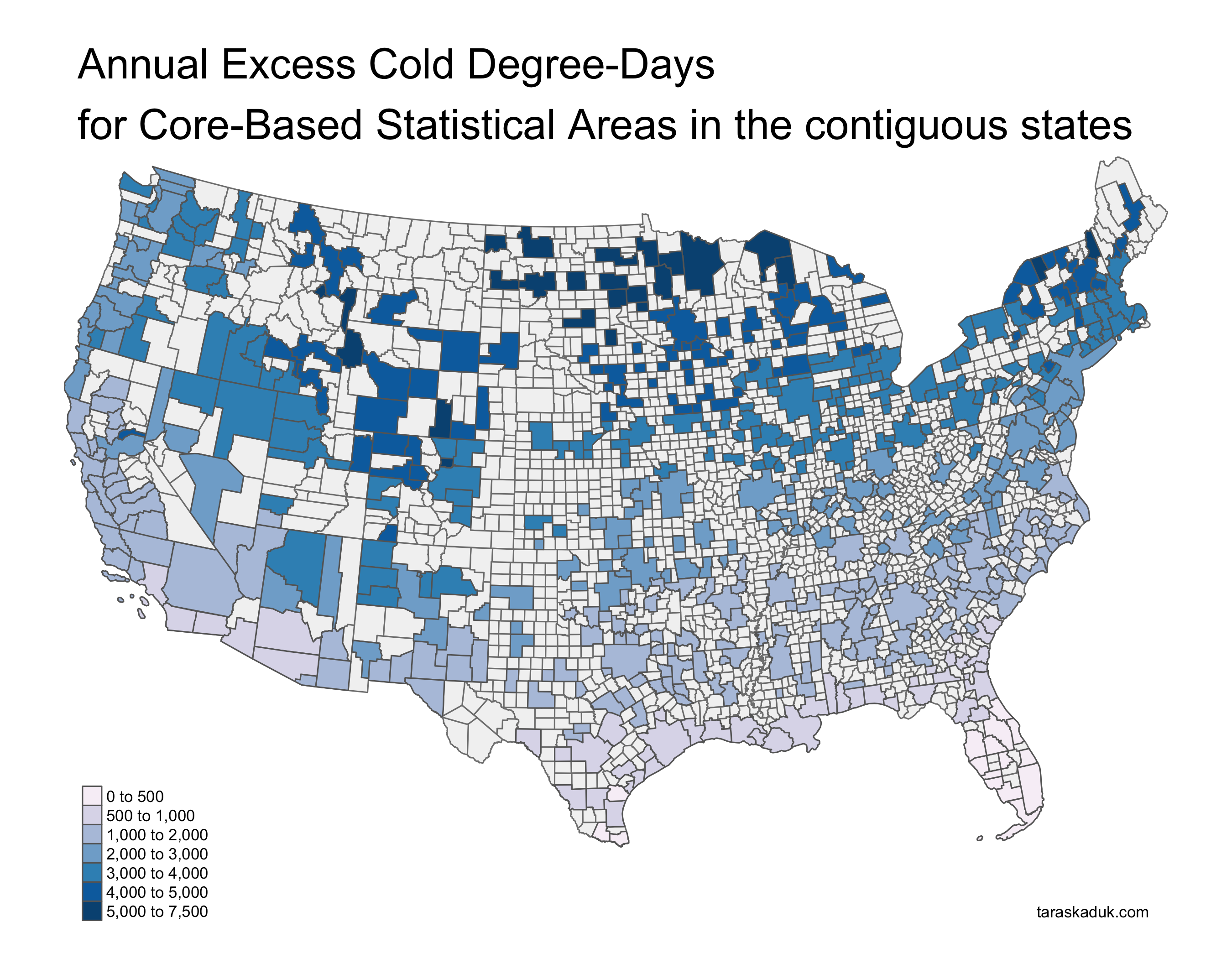
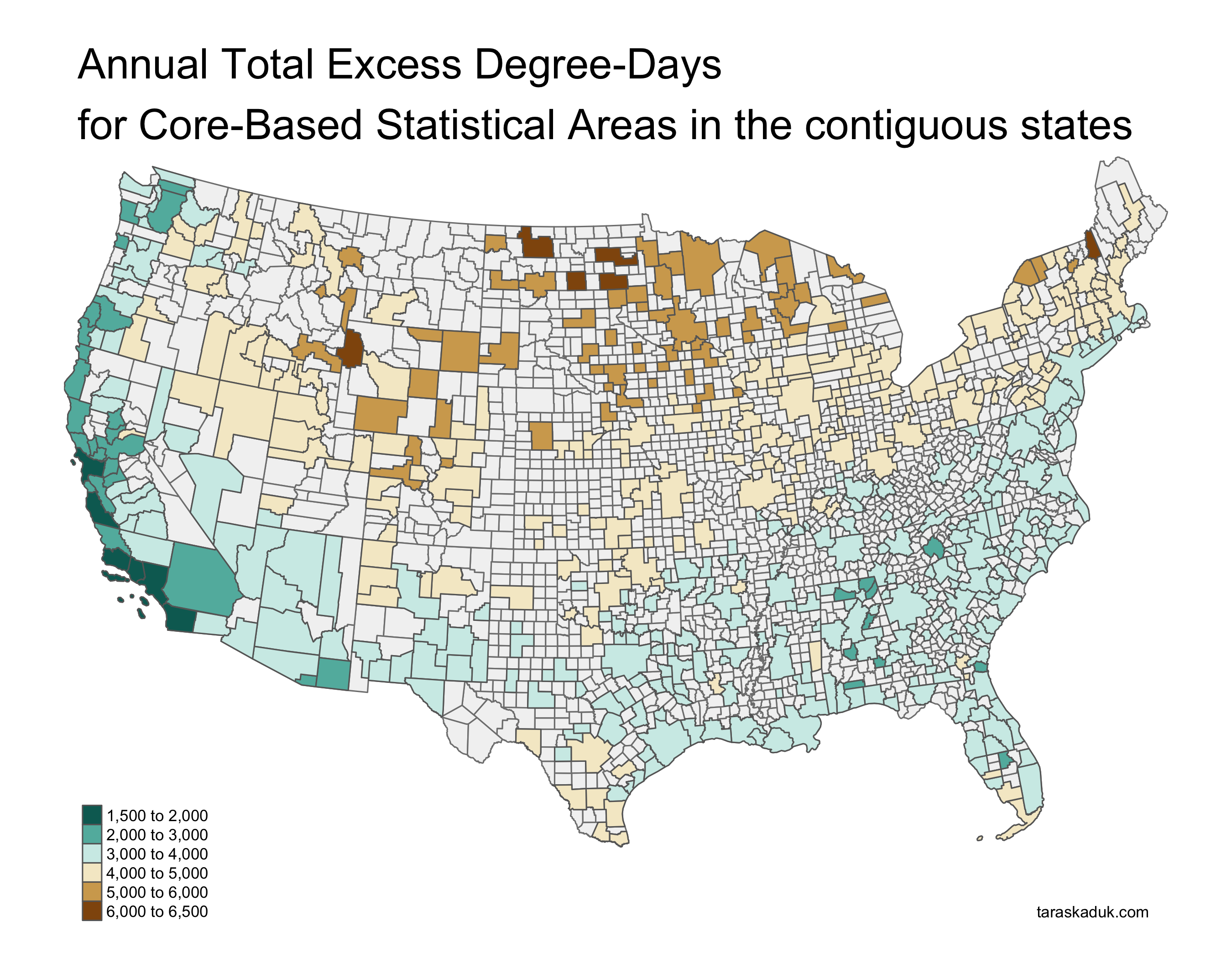
U.S. CBSAs ranked by excess degree-days

One quick demonstration of the EDD calculation can be done with displaying the EDD for the United States CBSAs. I will use the data from another project I’ve been working on:⁴

The way these figures are represented spatially can be visualized as follows:

Notes

Initial tweet shortly after I came up with the calculation idea following looking at weather data and solving integral equations:

That calculus class finally comes in handy. Figuring out a better way to measure a day’s pleasant air temperature through integration. Pretty excited about this one. pic.twitter.com/EIrXdBrHxV
— Taras Kaduk (@taraskaduk) May 2, 2019

R code for EDD

Here is the R function to obtain the area between the temperature curve and the baseline. This function can be used in a data frame (adhering to the tidy data analysis framework) and applied with a purrr::map2_dbl() call inside a mutate() call.

require(tibble)

get_edd <- function(min, max, baseline = 18) {
  
  # First, create the temp. function:
  a <- (max-min)/2 #amplitude
  period <- 24
  b <- 2 * pi / period
  d <- min + a
  
  # This is our temperature function:
  temperature <- function(x) {
    -a * cos(b * x) + d
  }
  
  
  # 3 calculations based on the 3 scenarios
  # of how the curve and the baseline interact
  
  if (min >= baseline) {
    # integral <- -a*sin(24*b) + 24*d - 24*baseline
    integral <- integrate(temperature, 0, 24)$value - baseline * 24 %>% 
      round(2)
    edd <- tibble( edd_hot = round(integral/24,2),  
                   edd_cold = 0, 
                   edd_total = round(integral/24,2))
    
  } else if (max <= baseline) {
    integral <- baseline * 24 - integrate(temperature, 0, 24)$value %>% 
      round(2)
    
    edd <- tibble( edd_hot = 0,  
                   edd_cold = round(integral/24,2), 
                   edd_total = round(integral/24,2))
    
  } else {
    intercept1 <- acos((d - baseline) / a) / b
    intercept2 <- (12 - intercept1) * 2 + intercept1
    
    integral1 <-
      baseline * intercept1 - integrate(temperature, 0, intercept1)$value
    
    integral2 <-
      integrate(temperature, intercept1, intercept2)$value - baseline * (intercept2 - intercept1) 
    
    integral3 <-
      baseline * (24 - intercept2) - integrate(temperature, intercept2, 24)$value 
    
    edd <- tibble(edd_hot = round(integral2/24,2),  
                   edd_cold = round((integral1 + integral3)/24,2), 
                   edd_total = round((integral1 + integral2 + integral3)/24,2))
  }
  return(edd)
}

Chow, D. H. C., and Geoff J. Levermore. 2007. “New Algorithm for Generating Hourly Temperature Values Using Daily Maximum, Minimum and Average Values from Climate Models.” Building Services Engineering Research and Technology 28 (3): 237–48. https://doi.org/10.1177/0143624407078642.

Climate Impact Lab. 2018. “Estimating the Frequency of 90 Degree Days.” https://www.impactlab.org/wp-content/uploads/2018/08/CIL_Days-over-90_Method.pdf.

Lin, Qiaoxuan, Hualiang Lin, Tao Liu, Ziqiang Lin, Wayne R. Lawrence, Weilin Zeng, Jianpeng Xiao, et al. 2019. “The Effects of Excess Degree-Hours on Mortality in Guangzhou, China.” Environmental Research 176 (September): 108510. https://doi.org/10.1016/j.envres.2019.05.041.

Livingston, Ian. 2020. “Washington Breaks Record for Most 90-Degree Days in a Month.” Washington Post, July. https://www.washingtonpost.com/weather/2020/07/27/washington-dc-july-record-heat/.

Megyesi, M. S., S. P. Nawrocki, and N. H. Haskell. 2005. “Using Accumulated Degree-Days to Estimate the Postmortem Interval from Decomposed Human Remains.” Journal of Forensic Science 50 (3): 1–9. https://doi.org/10.1520/JFS2004017.

Plumer, Brad, and Nadja Popovich. 2017. “95-Degree Days: How Extreme Heat Could Spread Across the World.” The New York Times, June. https://www.nytimes.com/interactive/2017/06/22/climate/95-degree-day-maps.html, https://www.nytimes.com/interactive/2017/06/22/climate/95-degree-day-maps.html.

Thom, H. C. S. 1952. “Seasonal Degree-Day Statistics for the United States.” Monthly Weather Review 80 (9): 143–47. https://doi.org/10.1175/1520-0493(1952)080<0143:SDSFTU>2.0.CO;2.

Zalom, FG, PB Goodell, LT Wilson, WW Barnett, and Bentley, WJ. 1983. “Degree Days: The Calculation and Use of Heat Units in Pest Management. University of California. Division of Agriculture and Natural Resources Leaflet.” University of California Division of Agriculture and Natural Resources Leaflet 21373.

I was not aware of such computations until after writing out the logic of it. I came up with the idea independently while looking into weather patterns across U.S. cities, while simultaneously auditing a Calc III class for a refresher. My understanding is that it is best practice to cite similar research even if it was not used in researching or writing the paper.↩︎
This assumption only requires 2 data inputs (min and max daily temperature) instead of continuous temperature reading.↩︎
This assumption helps us in modeling the curve without any additional inputs, while a more precise approach would require sunrise, sunset, and solar noon times for each day (Chow and Levermore 2007)↩︎
https://taraskaduk.com/2019/02/18/weather/ for the write-up of the methodology, and https://github.com/taraskaduk/place-to-live for the data and the R code to obtain the data↩︎

Measuring Excess Degree-Days in the Context of Location Comfort and Liveability